I am a third-year PhD student in Population Health at University of Wisconsin-Madison. My advisor is Dr. Maureen Smith. I explore the association between telehealth use and unplanned events during COVID-19 and multilevel factors that may improve colorectal cancer screening rates at rural and urban clinics in Wisconsin, by working closely with Dr. Jessica Cao, Dr. Jennifer Weiss, and Dr. Guanhua Chen.
I was trained in computer vision, machine learning and natural language processing. I got my master’s degrees in Biomedical Data Science and Computer Science from University of Wisconsin-Madison and University of Connecticut, respectively. I received my bachelor’s degree in Electrical Engineering and Computer Science from Southeast University.
I am interested in trustworthy machine learning in healthcare. I would like to know if causal inference can help better understand machine learning models when focusing on health services research and clinical problems. With causal inference embedded, these black-box models may become more interpretable and generalizable, rather than being limited to finding patterns in the data.
Stat 888
Telehealth has been gradually equipped to the U.S. healthcare system in the past few decades [1], while we noticed that COVID-19 has triggered rapid expansion of telehealth [2-3] to reduce the risk of infection. In February 2020, the Centers for Disease Control and Prevention (CDC) issued guidance advising individuals and healthcare providers in areas affected by the COVID-19 pandemic to practice social distancing practices, specifically recommending that healthcare facilities and providers offer clinical services virtually such as telehealth. In March 2020, Centers for Medicare & Medicaid Services (CMS) announced initial telehealth flexibilities for Medicare beneficiaries, allowing the same payment level for telehealth as for in-person visits. [4]
However, there is limited evidence about the effects of telehealth on long-term patient outcomes. [5-6] Some people support telehealth due to its timely care access [7-8], while some argue that telehealth is not an adequate substitute for in-person visits, which can cause even more delayed or missed care, resulting in worse outcomes. [9-10] Uncertainty and debates have prevented the policymakers, insurers, healthcare providers and other entities to make permanent decisions on telehealth in the post-pandemic future. [11-13]
This formally raises the question: compared to in-person visits, are telehealth visits beneficial in improving patient outcomes, such as fewer hospitalizations?
Model the Problem
In order to simplify the problem, three random variables are defined for each invidual in this study.
- Treatment assignment \(A \in \{0, 1\}\), where \(A = 1\) indicates telehealth visits and \(A = 0\) indicates in-person visits. Each individual is assumed to choose telehealth or in-person services independent of the choice of others.
- Outcome \(Y \in N^0\), a non-negative integer, indicating the number of hospitalizations within 30 days of the visit.
- Patient characteristics \(X \in R^d\), a \(d\) real-valued vector, including patient sociodemographics and health conditions at baseline.
Sociodemographics contain age group (65-74 years old, 75-85, and 86+), gender (female/non-female), race/ethnicity (non-hispanic white/other), Medicaid enrollment (binary indicator), disability entitlement (binary indicator) and geographical residence (urban, suburban, large town, small town/isolated rural). The hierarchical condition categories (HCC) score and a binary indicator of having three or more chronic conditions serve as the description of patients’ health conditions.
Causal Effect
There is an underlying assumption to this question: sampled participants in the study are able to access telehealth services. However, telehealth is not available to everyone, such as those who do not have access to the Internet. Therefore, it is reasonable to define population average treatment effect \(E[Y(A = 1) - Y(A = 0) \mid S = 1]\) for this problem, where \(S \in \{0, 1\}\) and \(S = 1\) represents being sampled in this study.
Hypotheses
Ideally, the directed acyclic graph (DAG) can be as simple as \(A \rightarrow Y \leftarrow X\) since \(X\) precedes \(A\) and \(A\) precedes \(Y\), indicating both \(X\) and \(A\) can affect \(Y\) but pre-existing characteristics \(X\) and the treatment \(A\) cannot be affected by \(Y\). This also assumes that individuals receiving treatment \((A = 1)\) or not \((A = 0)\) are expected to be exchangeable, i.e., potential outcomes are independent from the treatment assignment.
However, confounding variables, such as patient demographics and health conditions at baseline, may affect their treatment assignment. Then it adds a path from \(X\) to \(A\), implying that there are two paths from \(X\) to \(Y\) in a single DAG: \(X \rightarrow A \rightarrow Y\) and \(X \rightarrow Y\) if assuming confounding variables are observed. Furthermore, if taking unobserved characteristics \(U \subseteq X\) into consideration as well, such as preferences for telehealth versus in-person services, then the DAG can contain two paths from \(U\) to \(Y\): \(U \rightarrow Y\) and \(U \rightarrow A \rightarrow Y\).
In practice, it seems reasonable to consider that unobserved characteristics \(U\) and observed characteristics \(C\) can influence each other, where \(X = C \cup U\). For example, preferences for telehealth versus in-person services may influence the geographic residence of participants, as those who prefer telehealth visits may tend to live in places with stable Internet access. However, some rural areas may have limited access to high-speed Internet. Meanwhile, rural residents may have less access to healthcare services, especially specialty care. [14] Telehealth is encouraged to overcome the geographic barriers faced by rural communities, which may influence people’s preferences for telehealth versus in-person at the time of visit. For simplicity of modeling, only the path from \(C\) to \(U\) is kept in the DAG and this raises an assumption to ignore the effect from \(U\) to \(C\). Then the path \(U \rightarrow A \rightarrow Y\) is updated to \(U \leftarrow C \rightarrow A \rightarrow Y\).
The relationship between the variables is summarized by a DAG as follows. 
Assumptions
- Exchangeability
Treatment assignment should be independent from potential outcomes to fulfill the exchangeability assumption, i.e., \(Y(a) \perp\kern-5pt\perp A\) for all \(a \in A\). However, it might be reasonable to assume conditional exchangeability within strata instead, while strata is supposed to be defined on those observed characteristics such as age, gender, race/ethnicity and geographical residence. As shown in the DAG, \(A\) and \(Y\) is d-separated by \(C\). Then we have \(Y(a) \perp\kern-5pt\perp A \mid C\) according to global Markov property. In other words, the assumption of conditional exchangeability within strata is satisfied.
It is also feasible to conduct matching to reduce the bias due to the confounding variables, to make exposed and non-exposed cohorts more comparable in the risk of developing the outcomes. Since it could be difficult to complete the matching process with several characteristics, propensity score matching is more appropriate based on observed explanatory variables, although it requires large sample size and it cannot deal with unobserved variables.
- Stable Unit Treatment Value Assumption (SUTVA)
SUTVA requires well-defined mapping from \(a\) to \(Y(a)\). It implies several assumptions, including consistency, treatment irrelevance, no interference and stochastic potential outcomes.
Consistency is assumed as \(Y = Y(a)\). In practice, those with more chronic conditions at baseline may tend to have more hospitalizations than those are healthier, although both groups receive the same treatment. Therefore, it seems better to assume consistency within strata, while strata is defined by the observed characteristics \(C\), or to introduce additional unobserved confounding variables instead.
Treatment irrelevance is assumed, so this study does not distinguish between subtypes in telehealth and in-person visits. For instances, audio, audio and video interactive, audio and video real-time interactive services are all considered telehealth visits. A similar idea applies to in-person visits. This can also be treated as a limitation of the data, since all telehealth visits are coded the same. Therefore, it is not possible to distinguish their subtypes from the collected data.
The assumption of no interference is satisfied. Patients are treated independently through telehealth or in-person visits and their potential outcomes are not expected to be affected by other individuals’ assignment to the intervention.
The assumption of stochastic potential outcomes is not a concern here since number of hospitalizations within 30 days is a one-time measure for each telehealth or in-person visit.
- Positivity
Individuals in this study are free to choose between telehealth and in-person services at each visit. Therefore, positivity is satisfied as \(P(A = a \mid C) \in (0, 1)\) for all \(a \in A\).
Identification
As shown in the DAG above, \(A\) and \(Y\) are d-separated by \(C\). Then we have \(E[Y(a) \mid C] = E[Y(a) \mid A = a, C]\) since \(Y(a) \perp\kern-5pt\perp A \mid C\).
The consistency assumption yields \(Y = Y(a)\). So, \(E[Y(a) \mid A = a, C] = E[Y \mid A = a, C]\).
In addition, \(E[Y(a)] = E[E[Y(a) \mid C]]\) due to the law of total expectation.
Combining the three expressions, \(E[Y(a)] = E[E[Y(a) \mid C]] = E[E[Y(a) \mid A = a, C]]\) \(= E[E[Y \mid A = a, C]]\). Hence, the identification is complete.
The proof affrims that appropriate \(A\), \(Y\) and \(C\) are needed to identify the causal effect of interest, under a series of assumptions mentioned earlier. If assuming each individual in the target population is equally likely to be sampled in this study, i.e., \(Y(a) \perp\kern-5pt\perp S\) for all \(a \in A\), then the defined population average treatment effect \(E[Y(A = 1) - Y(A = 0) \mid S = 1]\) \(= E[Y(A = 1) - Y(A = 0)] = E[Y(A = 1)] - E[Y(A = 0)] = E[E[Y \mid A = 1, C]]\) \(- E[E[Y \mid A = 0, C]]\) because of the linearity of expectation.
It goes without saying that which variables are expected to be aggregated to the observed characteristics \(C\) deserve further discussion given real data. Particularly, access to complete patient-level health care utilization based on electronic health records (EHRs) may be limited. Health insurance claims can act as supplement to EHRs [15] while their comprehensive and timely access may be a challenge for researchers. Therefore, two different sets of \(C\) and \(U\) can be defined depending on the availability of claims data: treat sociodemographics as observed variables and all health-related factors as unobserved variables if claims are not available; or treat sociodemographics and baseline care utilization as observed and other variables, such as preferences for telehealth versus in-person visits, as unobserved if claims are available. While both versions answer the research question above, the former effectively becomes a social inequality question, while the latter retains both sociodemographic and health-related factors to explore the causal relationship between treatment and outcome.
Estimation
I used inverse probability weighting (IPW) for estimation. It includes the following steps:
- Load data and remove missing values;
- Fit a logistic regression model to explain the treatment \(A\) as a function of all observed patient characteristics \(C\). Then its predictions through this fitted logistic regression is the estimated propensity score \(\hat{e}(C)\);
- Compute IPW estimators for those with \(A = 1\) and \(A = 0\) according to \(E[Y(1)] \approx E_N\left[\frac{AY}{\hat{e}(C)}\right]\) and \(E[Y(0)] \approx E_N\left[\frac{(1 - A)Y}{1 - \hat{e}(C)}\right]\), respectively;
- Compute the difference to get IPW estimate of average treatment effect (ATE) \(E[Y(1) - Y(0)]\).
Dataset
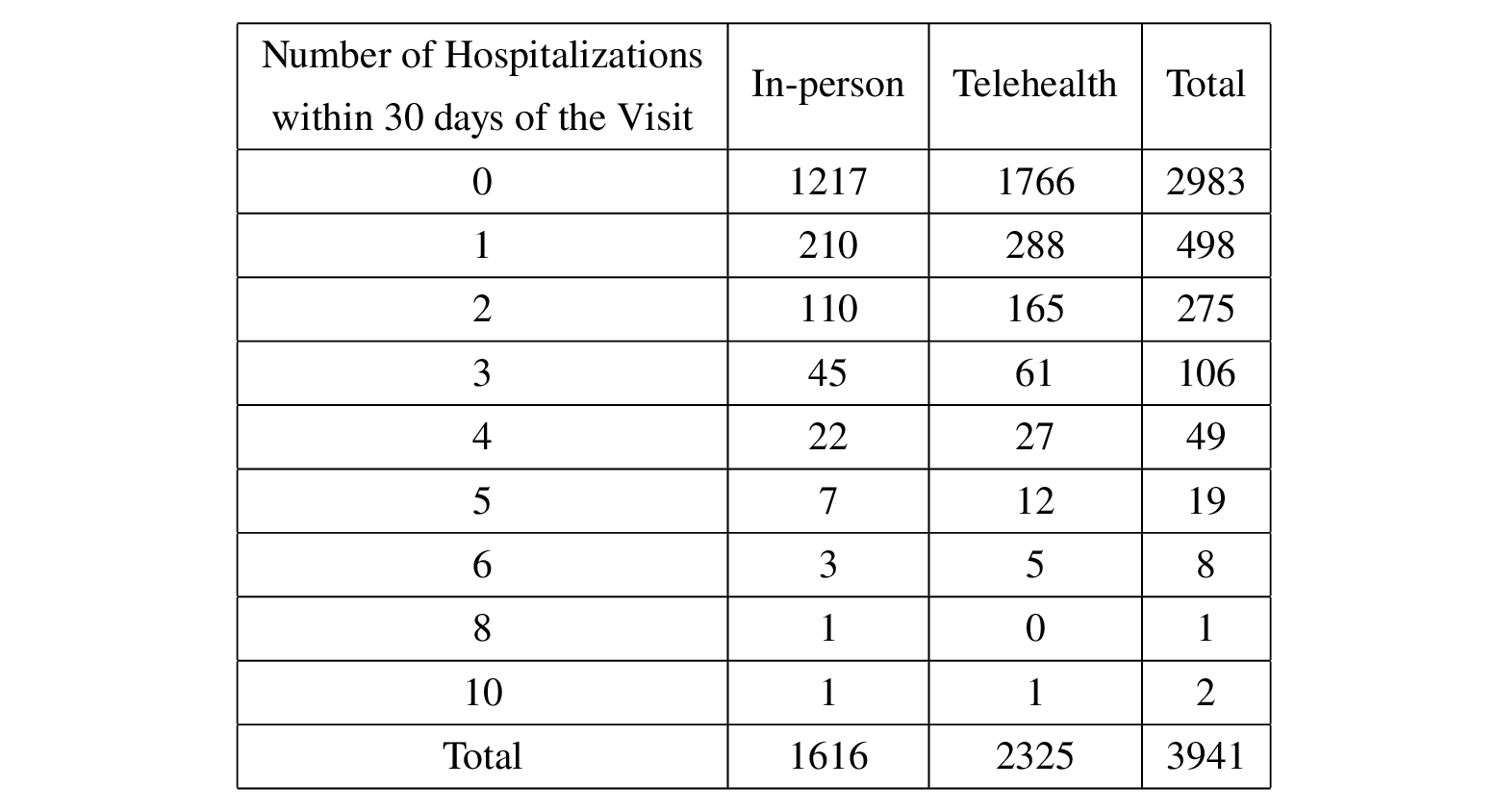
This study focuses on non-COVID outpatient care in primary care settings among Medicare beneficiaries served by an Accountable Care Organization (ACO) in southern Wisconsin. 3941 patients are included in the dataset. For simplicity, only their first visit after April 1, 2020 is included, for a total of 2325 telehealth visits and 1616 in-person visits as assigned treatment.
The number of hospitalizations within 30 days of this visit is counted as the outcome for each patient. 1375 patients did not have follow-up hospitalizations within 30 days of the visit, while 1225 patients had more than two follow-up hospitalizations within 30 days. Please see the table below for details. 
Variables are exactly the same as described in the Model the Problem section.
Discussion
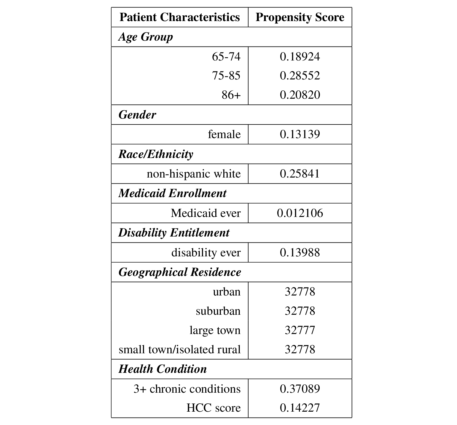
The estimated propensity scores are as follows. 
Then the IPW estimate of ATE is 0.044128 in this dataset. However, it can introduce bias if the estimation of propensity score is not perfect since \(E\left[E_N\left[\frac{1_{A = a}Y}{\hat{P}(A = a \mid X)}\right]\right] = E[Y(a)] + E\left[E[Y(a) \mid X]\frac{P(A = a \mid X)-\hat{P}(A = a \mid X)}{\hat{P}(A = a \mid X)}\right]\).
Therefore, I also tried augmented inverse probability weighting (AIPW) as it is doubly robust by combining IPW and outcome regression. The AIPW estimate of ATE is 0.047478, which is not much different from the IPW estimate. So we tend to conclude that telehealth leads to an increase in hospitalizations of about 0.044 to 0.047 within 30 days of the visit compared to in-person given this dataset.
As noted in class, both IPW and AIPW rely on observed variables to create propensity scores to balance between the treated and untreated groups. But unobserved variables may also affect the results, as described in the Hypotheses section. Then additional methods to address unmeasuresd confounding variables are expected for more accurate estimands.
Unmeasured Confounding
As described in the Discussion section above, only observed variables were considered when conducting IPW and AIPW, i.e., no unmeasured confounding variables were assumed.
Therefore, three alternative strategies were performed to take care of the unmeasured confounding: controlling for an additional variable (number of follow-up visits after the initial visit), Manski bounds and the E-value.
- Control for an additional variable
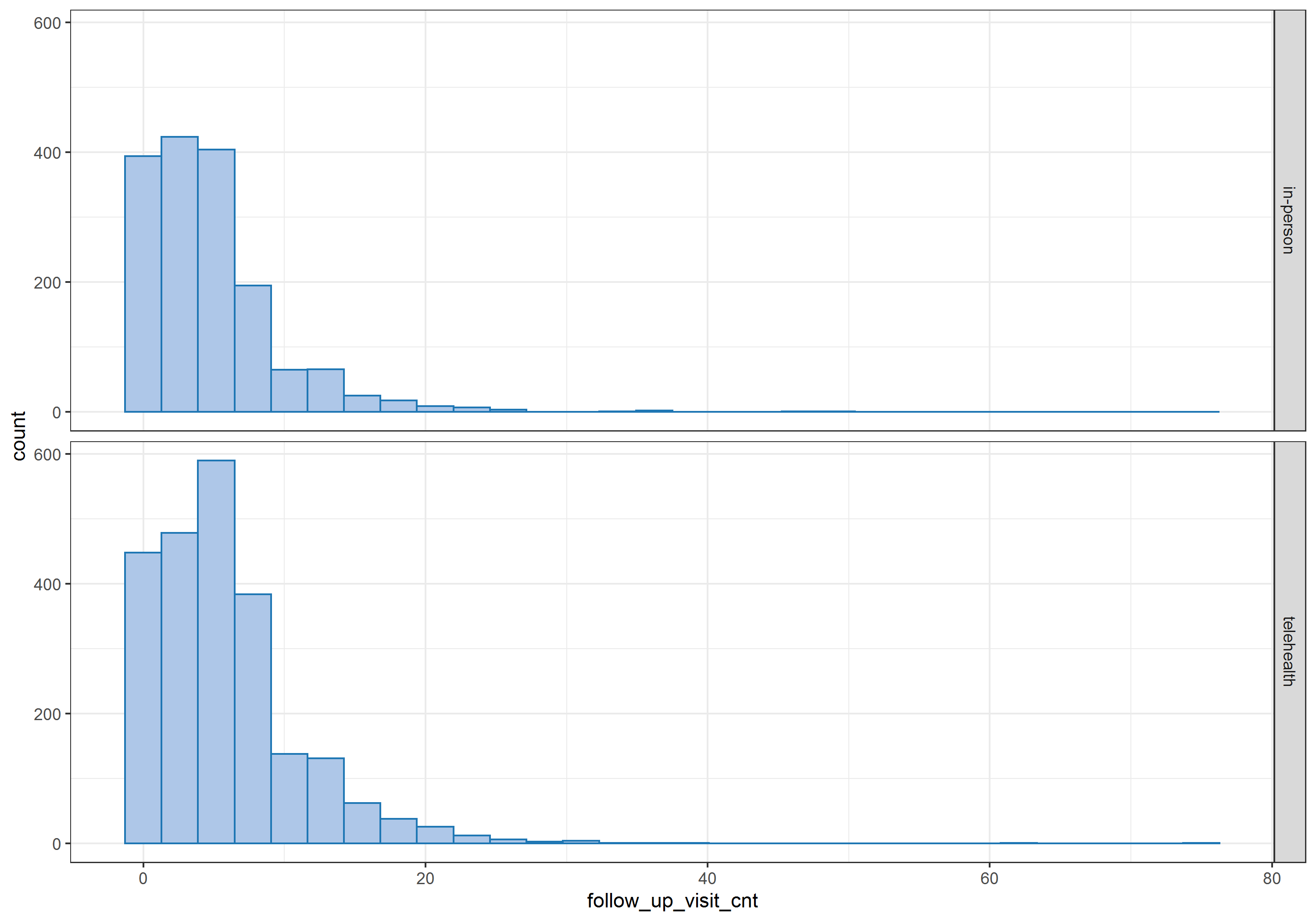
The number of follow-up visits after the initial visit (first visit after April 1st, 2020) varies from patient to patient, ranging from 0 to 75, as shown in the histogram below.  Therefore, I treated this additional variable as a proxy variable for patients’ unmeasured health status.
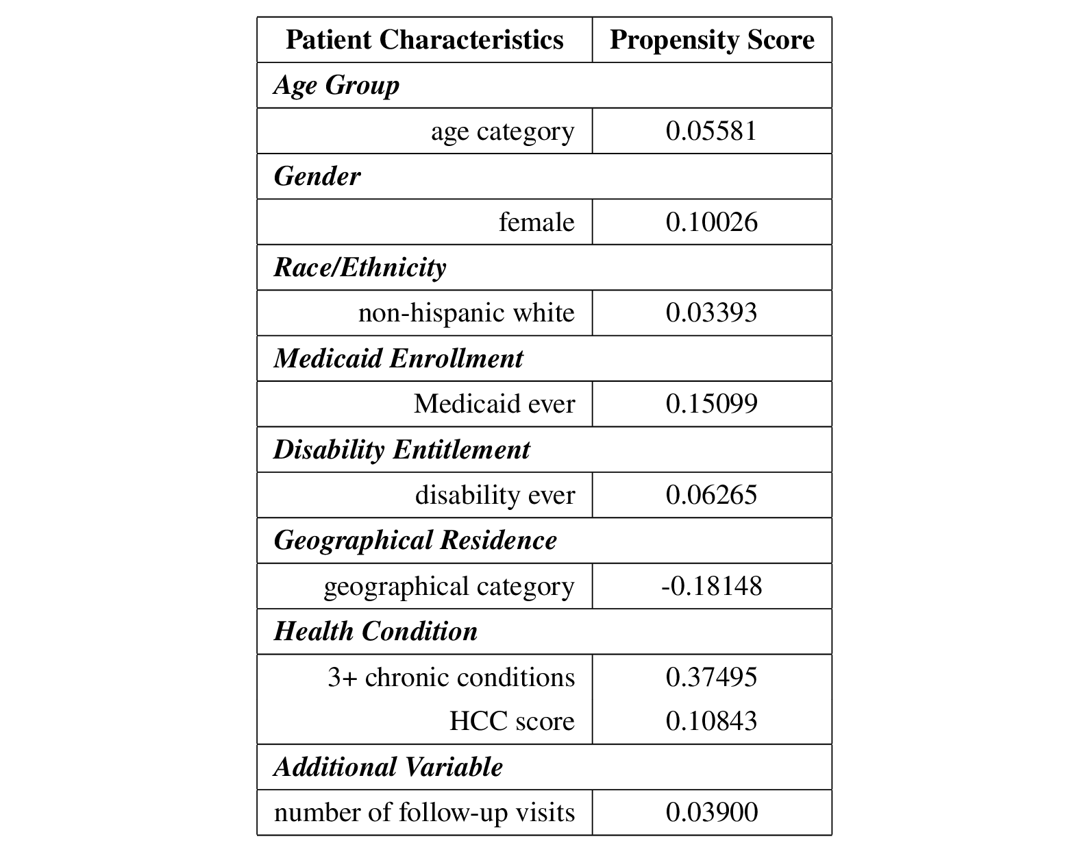
Repeating the IPW and AIPW estimates, coding age and geographical residence as categorical variables instead, the estimated ATEs became negative: -0.1164 for IPW and -0.10463 for AIPW, indicating that telehealth tends to lead a decrease in hospitalizations of about 0.10463 to 0.1164 within 30 days of the visit compared to in-person in this data. The conclusion is reversed when unmeasured confounders are not considered, as previous findings suggest that telehealth tends to increase the number of hospitalizations within 30 days of a visit, since the estimated ATE was about 0.044 to 0.047. Then it seems that the conclusion is sensitive to the violation of the assumption that there are no unmeasured confounders.
The following table summarizes the propensity scores after including the number of follow-up visits after the initial visit in the IPW and AIPW estimates. 
- Manski bounds
In the presence of unmeasured confounding, i.e., unobserved patient characteristics \(U\), Manski’s approach [16] is able to provide a bound for the estimated ATE, as the outcome \(Y\) is bounded by 0 and 10 in this dataset. Using the measurable portion of the ATE, I was able to obtained the Manski bounds: -5.8456 and 4.1544. This provides a range of the causal estimand in the presence of unmeasured confounding. However, this bounds may be less informative, as previous estimates of ATE were around -0.1 to 0.05.
The good news is that it seems reasonable to narrow the above bounds with additional monotonicity assumptions. As the focus of this study is on the first visit after April 1, 2020, and the number of hospitalizations within 30 days of the visit, it sounds reasonable that healthier individuals would tend to choose telehealth visits, while those with severe conditions may have to choose in-person visits since some medical exams lab tests cannot be performed without a patient on site. In addition, healthier individuals are expected to experience less hospitalizations compared to those with severe conditions due to their health status. In other words, it is reasonable to assume individuals’ number of hospitalizations would decrease if they choose telehealth visits compared to in-person visits, i.e., \(Y(1) \leq Y(0)\). Furthermore, it is also reasonable to assume that those who choose telehealth visits have fewer expected hospitalizations, regardless of their actual assigned treatment, i.e., \(E[Y(a) \mid A = 1, X = x] \leq E[Y(a) \mid A = 0, X = x]\).
Similar to the lecture notes, the above monotonicity assumptions give the proposition \(E[Y \mid A = 1, X] \leq E[Y \mid A = 0, X] \leq E[Y(1) - Y(0) \mid X] \leq 0\). Then I was able to computed the Manski bounds with the motonicity assumption based on the proposition. Its lower bound became -0.020721, which is much closer to the ATE estimated using IPW and AIPW. However, it appears impossible to check whether individual treatment responses are monotonic. The dependence on this untestable assumption is a limitation of this project.
- E-value
Another idea is the E-value, which provides the minimum strength of the association on the relative risk scale that unmeasured confounding would explain away the observed treatment-outcome association. [17] Calculated directly from the observed relative risk between the treatment \(A\) and the outcome \(Y\), the E-value quantifies how the unmeasured confounding can bias the treatment or the outcome while taking into account the associations of \(U \rightarrow Y\) and \(U \rightarrow A\).
After dichotomizing the outcome \(Y\) into a binary variable using the indicator function \(1_{Y > 0}\), a \(2\times 2\) table can be obtained as follows.  Therefore, the relative risk for the exposed group (\(A = 1\)) and the unexposed group (\(A = 0\)) is 0.9576 with 95% confidence interval (0.8500, 1.0787) and p-value 0.48. After taking the inverse of the relative risk (since it is protective) and applying the formula, the computed E-value is 1.2596 for the point estimate. However, the E-value for the confidence interval of the relative risk is 1 since the upper limit of the confidence interval is greater than 1. [18]
The E-value demonstrates that the unmeasured confounding increases the likelihood of the outcome by 1.2596, or the treatment increases the likelihood of the unmeasured confoundering by 1.2596, would explain away the observed relative risk of 0.9576 for the treatment-outcome association. Although this small E-value suggests weak evidence of causality, it describes how strong the umneasured confounding would relate to the observed treatment-outcome association.
Conclusion
In this project, I explored whether people who opted for telehealth tended to have fewer hospitalizations within 30 days of their visits compared to those who opted for in-person visits. The results showed that telehealth tended to reduce hospitalizations by approximately 0.1 after adjusting for patient characteristics, health conditions at baseline, and number of follow-up visits after the initial visit. In addition, there was weak evidence of a causal relationship between choice of telehealth or in-person visits and the number of hospitalizations, with E-value is 1.2596. Unfortunately, I was not able to test the monotonicity assumption to narrow down the bounds of unmeasured confounding.
The focus of this work was on initial visits after April 1, 2020 and their subsequent hospitalizations. However, due to the pandemic, especially for this early stage of COVID-19, there may be some missed or delayed care, resulting in inaccurate or even biased data. It is also possible that the visit was not related to the subsequent hospitalization, for example, a visit for flu while a hospitalization for a car accident, making the causal relationship between the visit and the hospitalization inherently weak, while reasons for visits and hospitalizations are absent in this dataset.
Reference
[1] Jagarapu, Jawahar, and Rashmin C. Savani. “A brief history of telemedicine and the evolution of teleneonatology.” In Seminars in Perinatology, vol. 45, no. 5, p. 151416. WB Saunders, 2021.
[2] https://www.cdc.gov/mmwr/volumes/69/wr/mm6943a3.htm
[4] https://www.medicare.gov/coverage/telehealth
[5] Goldberg, Elizabeth M., Frances N. Jiménez, Kevin Chen, Natalie M. Davoodi, Melinda Li, Daniel H. Strauss, Maria Zou, Kate Guthrie, and Roland C. Merchant. “Telehealth was beneficial during COVID‐19 for older Americans: a qualitative study with physicians.” Journal of the American Geriatrics Society 69, no. 11 (2021): 3034-3043.
[6] https://www.healthaffairs.org/do/10.1377/forefront.20211019.985495/
[7] Johnson, Pamela Jo, Neha Ghildayal, Andrew C. Ward, Bjorn C. Westgard, Lori L. Boland, and Jon S. Hokanson. “Disparities in potentially avoidable emergency department (ED) care: ED visits for ambulatory care sensitive conditions.” Medical care (2012): 1020-1028.
[8] Lee, Ivy, Carrie Kovarik, Trilokraj Tejasvi, Michelle Pizarro, and Jules B. Lipoff. “Telehealth: Helping your patients and practice survive and thrive during the COVID-19 crisis with rapid quality implementation.” Journal of the American Academy of Dermatology 82, no. 5 (2020): 1213-1214.
[9] Bavafa, Hessam, Lorin M. Hitt, and Christian Terwiesch. “The impact of e-visits on visit frequencies and patient health: Evidence from primary care.” Management Science 64, no. 12 (2018): 5461-5480.
[10] Li, Kathleen Y., Sophia Ng, Ziwei Zhu, Jeffrey S. McCullough, Keith E. Kocher, and Chad Ellimoottil. “Association Between Primary Care Practice Telehealth Use and Acute Care Visits for Ambulatory Care–Sensitive Conditions During COVID-19.” JAMA network open 5, no. 3 (2022): e225484-e225484.
[12] Shachar, Carmel, Jaclyn Engel, and Glyn Elwyn. “Implications for telehealth in a postpandemic future: regulatory and privacy issues.” Jama 323, no. 23 (2020): 2375-2376.
[13] Bashshur, Rashid L., Charles R. Doarn, Julio M. Frenk, Joseph C. Kvedar, Gary W. Shannon, and James O. Woolliscroft. “Beyond the COVID pandemic, telemedicine, and health care.” Telemedicine and e-Health 26, no. 11 (2020): 1310-1313.
[14] Mueller, J. Tom, Kathryn McConnell, Paul Berne Burow, Katie Pofahl, Alexis A. Merdjanoff, and Justin Farrell. “Impacts of the COVID-19 pandemic on rural America.” Proceedings of the National Academy of Sciences 118, no. 1 (2021): 2019378118.
[15] Smith, Maureen A., Mary S. Vaughan-Sarrazin, Menggang Yu, Xinyi Wang, Peter A. Nordby, Christine Vogeli, Jonathan Jaffery, and Joshua P. Metlay. “The importance of health insurance claims data in creating learning health systems: evaluating care for high-need high-cost patients using the National Patient-Centered Clinical Research Network (PCORNet).” Journal of the American Medical Informatics Association 26, no. 11 (2019): 1305-1313.
[16] Manski, Charles F. “Nonparametric bounds on treatment effects.” The American Economic Review 80, no. 2 (1990): 319-323.
[17] Ding, Peng, and Tyler J. VanderWeele. “Sensitivity analysis without assumptions.” Epidemiology (Cambridge, Mass.) 27, no. 3 (2016): 368.
[18] VanderWeele, Tyler J., and Peng Ding. “Sensitivity analysis in observational research: introducing the E-value.” Annals of internal medicine 167, no. 4 (2017): 268-274.
